class: center, middle, inverse, title-slide # Colocalization: Spatial Point Analysis ## NEUS 643 ### Ted Laderas ### 2020-05-26 --- # Learning Objectives - Understand the roots of spatial point analysis - Learn about *Density* measures - Learn about *Average Nearest Neighbor* and its cross version - Learn about *Ripley's K* and its cross version - Learn about *Complete Spatial Randomness* - Interpret envelope plots of both *Ripley's K* and *ANN* --- # Caveat Many of these methods are brand new to microscopy. Thus, many of them aren't implemented in software, or very well. They come from spatial analysis and geography. --- # Object Based Colocalization - We've extracted features from our images - Can we do better statistics with the features than just correlation? --- # Starting point: X and Y coordinates 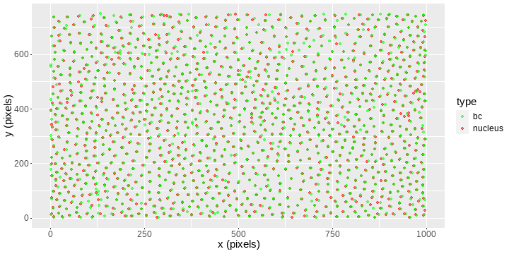<!-- --> ??? The starting point for spatial analysis are the x and y coordinates of our features. Each of these features can have a *mark*. In our case the marks are from the Red and Green Channels. --- # Window of Sampling - Need to specify the window of sampling - Changes aspects of the modeling --- # What is our range of interest? - Need to define this explicitly - Calculate metrics over this range of interest - Compare to outside of this range --- # Concepts: First order versus Second Order <img src="image/week8/1st_2nd_order_property.png" width = 800> ??? This figure again is from geography, but we can talk about first order properties - properties dependent on the geographical properties, such as chemical gradient second order properties - properties dependent on neighbors --- # Discussion - What are some 1st order properties in microscopy of cells? - What are some 2nd order properties in microscopy of cells? --- # Concepts: Density - Can be *global* or *locally* calculated - Often a good first exploration of the data --- #Local Density: Quadrat 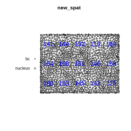<!-- --> --- #Local Density: Density Plot 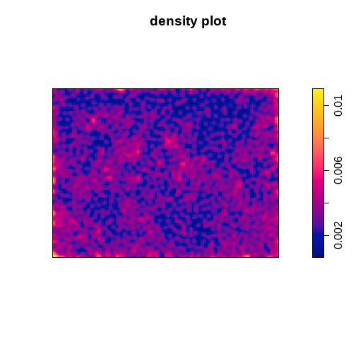<!-- --> --- # Concepts: Distance - Euclidean distance between point that is nearest to a point - Find all neareset neighbors --- <img src="image/week8/ann1.JPG" width=800> --- # Average Nearest Neighbor (ANN) <img src="image/week8/f11-ppp-dist-1.png" height=500> ??? --- # Order plot <img src="image/week8/f11-ANN-plot-1.png"> ??? The order plot can often give us clues about the structure. --- # The shape of the order plot <img src="image/week8/f11-diff-patterns-1.png" height=230 > <img src="image/week8/f11-diff-ANN-plots-1.png" height=230> ??? You can see that the shape --- <img src="image/week8/ann_cross.JPG" width = 800> --- <img src="image/week8/ripleyK1.JPG" width=800> --- <img src="image/week8/ripleyK.JPG" width=800> --- <img src="image/week8/ripleyK_cross.JPG" width =800> --- class: center, middle # Where do the statistics come from? --- # Complete Spatial Randomness <img src = "image/week8/IRP_CSR.png" height = 500> ??? The null distributions we usually compare our data set to adhere to "Complete Spatial Random" Our *process* of generating the CSR data is independent, with proteins popping up in random spots Obviously, biological processes of cell growth are different, which suggests we probably need a good way of generating a random distribution that models this process. No one has gone there yet. --- <img src="image/week8/colocalized_null.jpg" height = 500> ??? http://wwwf.imperial.ac.uk/~eakc07/QBItalk.pdf Here we compare our two channels, on the left both channels have been generated by a CSR process. --- # Expected versus Observed - *Observed* - the observed value of our statistic for our data - *Expected* (or *Theoretical*) - the value of our statistic calculated under null distribution - Complete Spatial Randomness --- # Alternative Versus Null - Ha: The observed value and theoretical values are not identical - Ho: The observed value and theoretical values are identical --- # Generate Random Datasets 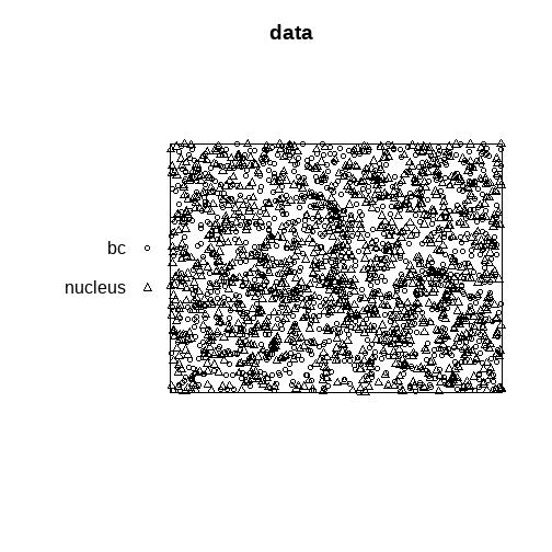<!-- --> ??? We can generate random data under the null hypothesis --- # Ripley's K ``` ## Function value object (class 'fv') ## for the function r -> K(r) ## .............................................................. ## Math.label Description ## r r distance argument r ## theo K[pois](r) theoretical Poisson K(r) ## border hat(K)[bord](r) border-corrected estimate of K(r) ## trans hat(K)[trans](r) translation-corrected estimate of K(r) ## iso hat(K)[iso](r) isotropic-corrected estimate of K(r) ## .............................................................. ## Default plot formula: .~r ## where "." stands for 'iso', 'trans', 'border', 'theo' ## Recommended range of argument r: [0, 187.5] ## Available range of argument r: [0, 187.5] ``` --- # Calculate over all fake datasets ```r test <- envelope(new_spat, Kcross, nsim=1000, r=c(0,30)) ``` ``` ## Generating 1000 simulations of CSR ... ## 1, 2, 3, ......10.........20.........30.........40.........50.........60........ ## .70.........80.........90.........100.........110.........120.........130...... ## ...140.........150.........160.........170.........180.........190.........200.... ## .....210.........220.........230.........240.........250.........260.........270.. ## .......280.........290.........300.........310.........320.........330.........340 ## .........350.........360.........370.........380.........390.........400........ ## .410.........420.........430.........440.........450.........460.........470...... ## ...480.........490.........500.........510.........520.........530.........540.... ## .....550.........560.........570.........580.........590.........600.........610.. ## .......620.........630.........640.........650.........660.........670.........680 ## .........690.........700.........710.........720.........730.........740........ ## .750.........760.........770.........780.........790.........800.........810...... ## ...820.........830.........840.........850.........860.........870.........880.... ## .....890.........900.........910.........920.........930.........940.........950.. ## .......960.........970.........980.........990......... 1000. ## ## Done. ``` ??? We can generate our null distribution using this process. We calculate it over a range of radii from 0 pixels to 30 pixels --- <!-- --> ??? The grey band represents the null distribution of K at different radi for datasets randomly generated under CSR. We look at our observed line, and notice that it's outside of the null distribution. Thus K is greater than expected over the range of 0-30 pixels --- # Generate for ANN ```r gc <- envelope(new_spat, Gcross) ``` ``` ## Generating 99 simulations of CSR ... ## 1, 2, 3, 4, 5, 6, 7, 8, 9, 10, 11, 12, 13, 14, 15, 16, 17, 18, 19, 20, 21, 22, 23, 24, 25, 26, 27, 28, 29, 30, 31, 32, 33, 34, 35, 36, 37, 38, 39, 40, ## 41, 42, 43, 44, 45, 46, 47, 48, 49, 50, 51, 52, 53, 54, 55, 56, 57, 58, 59, 60, 61, 62, 63, 64, 65, 66, 67, 68, 69, 70, 71, 72, 73, 74, 75, 76, 77, 78, 79, 80, ## 81, 82, 83, 84, 85, 86, 87, 88, 89, 90, 91, 92, 93, 94, 95, 96, 97, 98, 99. ## ## Done. ``` ??? There is a related metric to Average nearest neighbor called G. We generate a new distribution. --- # Average Nearest Neighbor Statistics <!-- --> The plot for G is similar to our order plot, but with the band representing the null distribution. We see across the 1st to 5th orders, the value of our G is greater than the theoretical G, which suggests colocalization across these orders. --- # Reporting colocalization - Must always report within a range --- # Nearest Neighbor Distances (percentage) .pull-left[ 48 percent of bc cells had a nearest neighbor of nucleus within 10 pixels ] .pull-right[ <!-- --> ] --- # Still trying to understand this <img src="image/week8/augh.jpg" width = 800> --- # Lab - Working with `spatstat` package - Generating Complete spatial random data - Working with Ripley's K and Average Nearest Neighbor --- # Reading - [Point Pattern Analysis](https://mgimond.github.io/Spatial/point-pattern-analysis.html) - [Hypothesis Testing](https://mgimond.github.io/Spatial/hypothesis-testing.html) - [Point Pattern Analysis in R](https://mgimond.github.io/Spatial/point-pattern-analysis-in-r.html)